My First Program Was Chaos

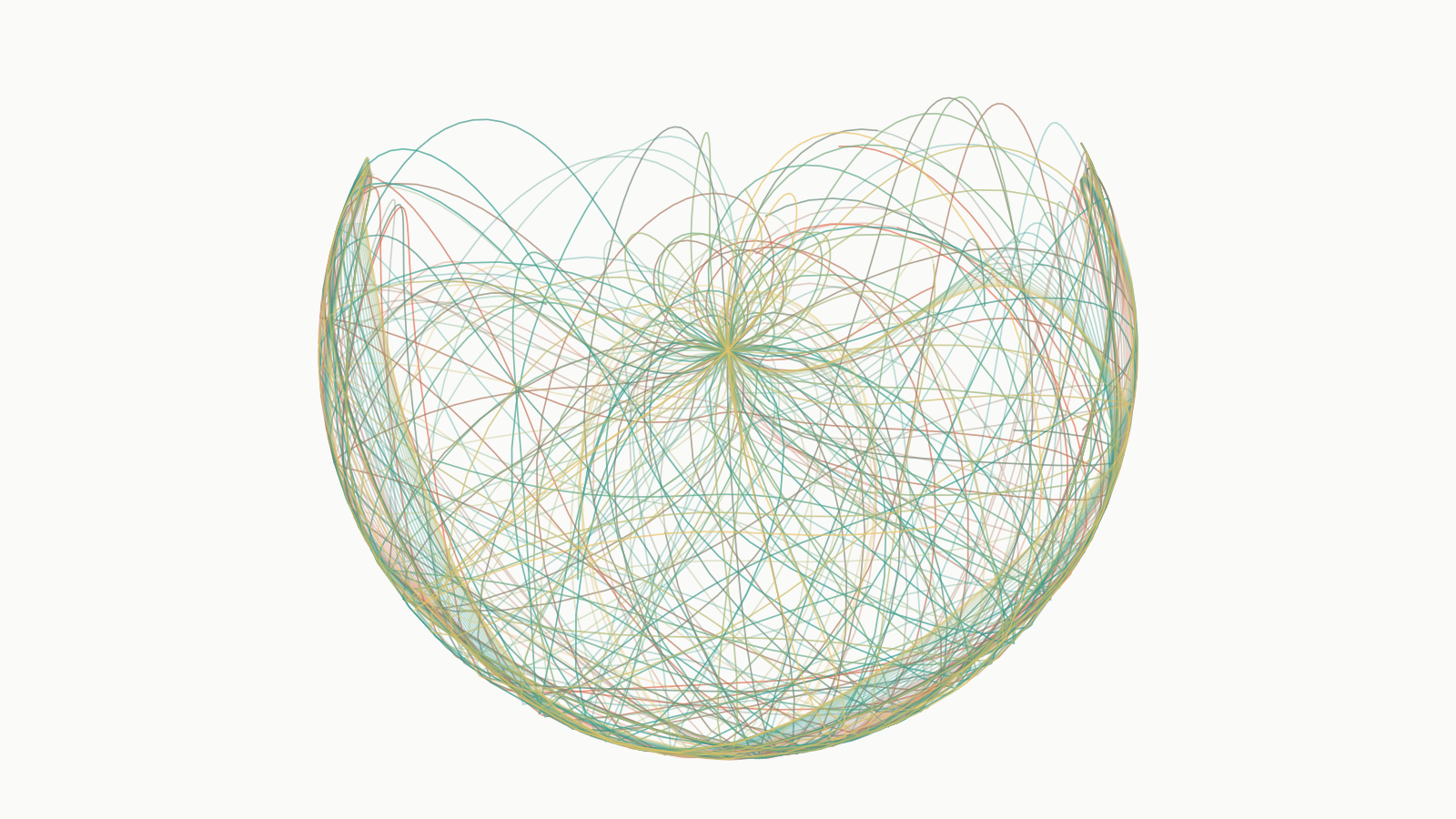
The first program I ever wrote was a double pendulum simulation. Not hello world, not FizzBuzz — a chaotic mechanical system, integrated in real time, in a browser. That sounds far more impressive than it was. It was 2016, I had just discovered Daniel Shiffman's Coding Train, and Coding Challenge #93 was a double pendulum in p5.js. I typed along, character for character, the way you copy out a recipe in a language you don't speak.

The heart of that sketch was a pair of acceleration formulas that Shiffman — openly, cheerfully — pasted from myphysicslab. Two fractions so long they wrapped across several lines of code: sines of sums and differences of angles, squared velocities feeding back into one another, one denominator repeated under both like a chorus. I understood none of it. Not the thetas, not the omegas, not whether that denominator could ever reach zero and take the sketch down with it. The pendulum didn't care. It swung, it flipped, the second bob traced those looping, never-repeating ribbons, and I sat there completely hooked and slightly bothered.

The bothered part never went away. I have been meaning to come back to this program for ten years, and this post is me finally doing it. This time we derive everything: the equations of motion from one principle and two energies, the reason the naive simulation explodes and the two-line accident that fixes it, what chaos means once you attach an actual number to it, and — last — a map of every possible double pendulum at once, which turns out to be a fractal. Every figure below is a live simulation. Drag them. That's what they're for.

One pendulum first

Before bolting two pendulums together, it pays to be honest about one. A single pendulum: a point mass $m$ on a rigid, massless rod of length $r$, swinging in a plane. One number pins down the entire configuration — the angle $\theta$ from the vertical.

You could solve this the Newtonian way: draw the force diagram, decompose gravity along and across the rod, and carry the rod's tension around as a bookkeeping variable even though it does no work and exists purely to keep the mass on its circle. That works. It is also exactly the kind of accounting that turns miserable the moment a system grows joints. So instead we use the tool that was built for jointed things — the Lagrangian:

kinetic energy minus potential energy, written in whatever coordinates genuinely describe the configuration. For us, that's $\theta$. The equation of motion then comes from turning a single crank, the Euler–Lagrange equation:

This is the condition for the trajectory to make the action — the time-integral of $L$ — stationary, and any mechanics text will tell that story properly. What matters for this post is the practical superpower: constraint forces never appear. The tension does no work, so it shows up in neither $T$ nor $V$. And because we chose $\theta$ as the coordinate, every motion we can even write down already keeps the mass on its circle. The constraint isn't enforced; it's built into the coordinate. Nothing to solve for, nothing to cancel.

Now the two energies. The bob moves at speed $r\dot{\theta}$, and — measuring $y$ downward from the pivot, a convention that keeps signs tidy for the rest of this post — it hangs at depth $r\cos\theta$:

Feed these through the crank: $\partial L/\partial \dot{\theta} = m r^2 \dot{\theta}$, differentiate that in time, subtract $\partial L/\partial \theta = -m g r \sin\theta$:

and divide through by $m r^2$:

Notice everything that didn't happen. No force diagram, no components, no tension. For one pendulum this saves five minutes. For two, it will save the whole derivation.

At this point every textbook plays the same trick: assume the swing is small, replace $\sin\theta$ with $\theta$, and the equation collapses into a harmonic oscillator you can solve outright:

A beautiful, load-bearing lie. The period doesn't depend on the amplitude — approximately — which is why pendulum clocks ruled timekeeping for three centuries. But it is strictly small print. Swing higher and the true period stretches. Push past the small-angle regime and the exact solution stops being expressible in elementary functions at all: you need elliptic integrals for one rod on one pivot. Remember that — it matters in a minute. Meanwhile, here is an honest pendulum next to its small-angle ghost:

Now bolt a pendulum to your pendulum

Hang a second rod and mass from the first bob. That is the entire modification. The configuration now needs two angles, $\theta_1$ and $\theta_2$, both measured from the vertical:

You are welcome to attempt the Newtonian route here. The tension in the second rod acts on both masses, along a direction that changes with both angles, while the first rod's tension responds to all of it at once — it's a classic exam problem precisely because the bookkeeping is punishing. The Lagrangian recipe doesn't flinch: same three steps, two coordinates. First, positions, with $y$ still measured downward from the pivot:

Bob 2 rides on bob 1: its position is bob 1's plus its own offset. That innocuous little sum is the whole story of this post. Differentiate in time, square, and add components to get speeds:

There it is: the cross term. How much bob 2's motion feeds off bob 1's depends on $\cos(\theta_1 - \theta_2)$, the alignment of the rods. Parallel rods add their velocities outright; perpendicular rods decouple; anti-parallel rods fight. Every ounce of trouble this system is about to cause traces back to that one cosine. The energies:

(Note the $m_1 + m_2$ in the first potential term: rod 1 carries both masses, so tilting it lifts both.) Now the crank, turned twice — once with $\theta_1$ as the coordinate, once with $\theta_2$. This is ten minutes of careful product-rule work, because the cross term depends on both angles and both angular velocities, so $d/dt$ keeps spawning $\sin(\theta_1 - \theta_2)$ terms that then partially cancel against the ones from $\partial L/\partial \theta$. If you want every intermediate line, Diego Assencio's derivation (linked below) writes them all out; I checked mine against his. Grouped and tidied, with the shorthand $\Delta = \theta_1 - \theta_2$, the two Euler–Lagrange equations assemble into a single matrix statement:

Read it left to right: a mass matrix — how hard the configuration resists angular acceleration, and note that it depends on $\Delta$, on where the pendulum currently is — times the accelerations, equals the applied torques: one centrifugal-flavored term from each bob's swing rate, plus gravity on each rod. It's Newton's second law wearing formal dress.

To simulate, we need the accelerations by themselves, which means solving that 2×2 system. Do it symbolically — Cramer's rule, substitute, expand — and out come two towering fractions, full of $\sin(\theta_1 - 2\theta_2)$ and $\cos(2\theta_1 - 2\theta_2)$, with one denominator repeated under both. Those fractions are, character for character, the myphysicslab formulas I pasted into p5.js in 2016. The monsters were never monsters. They are this one tidy matrix equation, pre-solved by hand and flattened into ASCII. It took me ten years to find that out.

Code doesn't need the flattened form — it just solves the little linear system numerically at every step. The only conceivable danger is that division: what if the determinant hits zero? It can't:

Since $\sin^2\Delta \ge 0$, the parenthesis is never smaller than $m_1$, which is positive because rod 1 carries an actual mass. (This is no accident — $M$ is the kinetic-energy metric, and kinetic energy is positive whenever anything moves.) The solve cannot blow up, for any angles, masses, or lengths. Which means we can safely hand it sliders:

Making it not explode

The matrix equation tells us the accelerations right now. A simulation needs the state later. Bridging that gap is numerical integration — and remember, even the single pendulum had no elementary closed-form solution, so numbers were always our destiny. The only question is how to step forward in time without lying too much. Pack the state into one vector:

where the $\omega$s are angular velocities and $f$ is everything we just derived: the rates of the angles are the $\omega$s, and the rates of the $\omega$s come from the matrix solve. Geometrically, $f$ is a velocity field on the four-dimensional state space, and our pendulum's entire life is one streamline of it. An integrator hops along that streamline in steps of size $h$. The obvious hop is explicit Euler — follow the tangent:

For a pendulum this is slow-acting poison, and the reason is geometric. Swinging motion loops around a closed orbit in state space — a level curve of the energy. The tangent to a loop points to the outside of the loop, so every Euler step lands slightly outside the orbit it left. Always outside, never inside: the errors don't cancel, they compound, and the trajectory spirals outward. For the small-angle oscillator you can prove each step multiplies the energy by $1 + h^2\omega^2$ — geometric growth. Your pendulum gains energy from nothing, every swing, until it's whipping around its pivot like a propeller.

You can watch this exact failure in the original Coding Train video: left alone, the sketch's pendulum slowly swings itself higher than it was dropped from. And the fix that ended up in the code — the fix I faithfully copied without a second thought — was simply to update the velocity first and then move the position using the new velocity:

Same arithmetic, same cost, two lines reordered. It looks like an off-by-one bug you decided to keep. It is actually a different algorithm with its own name — semi-implicit Euler, also sold as symplectic Euler — and a shockingly deep property: for systems whose energy separates cleanly into kinetic-of-velocity plus potential-of-position, like our single pendulum, it exactly conserves a slightly-perturbed "shadow" energy that sits within $O(h)$ of the true one. It cannot drift. Its energy error just oscillates in a bounded band, forever. By swapping two lines of JavaScript, Shiffman reached — presumably by accident — for one of the deepest results in numerical analysis.

Now the honesty footnote, because this is the detail everyone flattens: that ironclad guarantee is for separable systems, and the double pendulum is not one. The cross term ties kinetic energy to the angles — the mass matrix depends on $\theta$ — and with that, the strict symplectic warranty is void. What survives in practice is still remarkable: semi-implicit Euler's energy error creeps — slowly, first-order slowly — instead of staying in a fixed band, but it never runs away exponentially the way explicit Euler's does. Downgraded from "bounded forever" to "drifts politely." You can see exactly that downgrade in the demo below.

The third contender is the workhorse: classical fourth-order Runge–Kutta. Instead of committing to the slope at the start of the step, sample it four times — once at the start, twice at trial midpoints, once at a trial endpoint — and take a weighted blend:

where $k_1, \dots, k_4$ are those four slope samples, each evaluated where the previous one pointed. Fourth-order accuracy means halving $h$ cuts the error sixteen-fold. RK4 knows nothing about energy — run it for geological time and it too will drift — but at the step sizes used here its drift is negligible, which is why every other simulation on this page runs on it. Here are all three on the same pendulum, at the same time step:

The part where it becomes chaos

Everything so far — the derivation, the integrators, the energy audit — is the orderly half of the story. Here is the disorderly half, the half that kept a copied p5.js sketch lodged in my head for a decade. The equations above are perfectly deterministic: no randomness, no hidden inputs. Given the state exactly, the entire future is fixed. And the system is still unpredictable — in a precise, quantifiable, non-hand-wavy sense.

Run two copies of the pendulum, identical except for a nudge $\delta(0)$ in one angle — the kind of nudge a rounding error in the seventh decimal place would give you. Track the distance between them in state space. In the systems physics students are raised on, that distance grows politely: linearly, maybe quadratically. Here, it grows like this:

Exponentially — with $\lambda$, the Lyapunov exponent, as the system's built-in error-amplification rate: $1/\lambda$ is the time it takes an uncertainty to grow by a factor of $e$. On a log scale, exponential growth is a straight line, and you can watch that line draw itself in the demo below — a steady climb at slope $\lambda$, until the separation saturates because two pendulums can only get so far apart.

The consequence for prediction is brutal, and worth spelling out. Say you measure the initial state to some precision, and your forecast counts as good while the error stays under some tolerance. Then your horizon is

The logarithm is the villain. Measure a thousand times more precisely and the horizon grows by $\ln 1000 \approx 7$ units of $1/\lambda$ — a fixed few seconds for this pendulum, not a thousand times longer. Every additional digit of precision buys the same flat, modest increment of future. Determinism survives; prediction doesn't.

None of this is a pendulum quirk. Edward Lorenz met the same mathematics in the early 1960s in a stripped-down weather model, when a run restarted from printout values — rounded to three decimal places — invented an entirely different month of weather. That same logarithm is why forecasts stall out around two weeks no matter how good the satellites get: the atmosphere's $1/\lambda$ is a few days, and better data only ever buys logarithmically more horizon.

Every possible pendulum at once

Figure 6 asks about one pendulum and its nearest neighbors. The natural escalation is to ask about all of them. Fix the setup — equal masses and equal lengths, $m_1 = m_2 = m,\; r_1 = r_2 = l$, released from rest — so that a starting condition is nothing but a pair of angles $(\theta_1, \theta_2)$. Then ask every start the same question, Jeremy Heyl's question: how long until your second bob flips over the top? Color each pixel of the angle–angle plane by its answer, and you get the map in Figure 7 — my favorite picture in this entire subject.

Before simulating tens of thousands of pendulums, though, theory gets one more word, and it's a good one. Released from rest, the kinetic energy is zero, so the total energy is the starting potential:

(the 2 because rod 1 carries both masses). To flip, the pendulum must at some instant pass through a configuration with the second bob over the top, $\theta_2 = \pi$. Among all such configurations, the cheapest has bob 1 hanging straight down — $\theta_1 = 0$ — with potential $-mgl\,(2 - 1) = -mgl$. Energy is conserved and kinetic energy can't go negative, so if $E < -mgl$, every flipped configuration is out of reach. Forever. Unpacking the inequality:

Four lines of energy bookkeeping just proved a theorem about eternity: a pendulum released with $2\cos\theta_1 + \cos\theta_2 > 1$ — both rods hanging low — will never flip, no matter how long you wait. (You'll often see this quoted as $3\cos\theta_1 + \cos\theta_2 > 2$; that is the identical argument run for a compound pendulum built from uniform bars — Heyl's version — where the distributed mass shifts the coefficients.)

On the map below, that inequality is the black curve, and the pale region inside it is painted without simulating a single step. Outside it, chaos speaks: solid basins where the pendulum flips almost immediately, and — hugging the boundary — filigree where neighboring pixels flip after wildly different times, structure inside structure as far down as you care to zoom. That's Figure 6 restated as geography: near the boundary, "arbitrarily close starts, arbitrarily different fates" stops being a warning label and becomes a texture.

The theorem is also a computational free lunch. A pixel that never flips is the most expensive pixel there is — it burns the entire budget, thirty simulated seconds at 120 RK4 steps per second, just to answer "never" — and the inequality hands us about thirty percent of the map, precisely the pixels that would have cost the most, for free. Theory does the heavy lifting; the worker threads mop up.

Here's the part that gets me, ten years later. The 2016 sketch and this entire page run on the same hundred-ish lines of physics. The matrix solve driving every figure above is the myphysicslab formulas, un-flattened; the integrators are the same handful of additions and multiplications, ordered with intent. Nothing became more powerful. What changed is that every line is now load-bearing: I know why there's a $\cos(\theta_1 - \theta_2)$ in the kinetic energy, why the denominator that worried me can never reach zero, why swapping two updates tamed the energy drift, and why that trick's warranty quietly expired the moment we attached the second rod. The incantation became an argument.

If you have a formula like that — one you've been copying since before you could read it, someone else's variable names fossilized inside it — I can report that going back for it is worth the trip. Mine took ten years and turned into the five toys on this page. Scroll back up and drag the pendulums around one more time. That's still the whole point.

References

• Daniel Shiffman, The Coding Train — Coding Challenge #93: Double Pendulum. Where all of this started.
• myphysicslab — Double Pendulum. The hand-solved equations of motion I pasted in 2016, with their own full derivation.
• Daniel Shiffman — The Nature of Code. The book-length version of the sensibility that this post grew from.
• Diego Assencio — Double pendulum: Lagrangian formulation. Every intermediate step of the derivation, written out.
• Jeremy S. Heyl — The Double Pendulum Fractal (2008). The flip-time map, for the compound (uniform-bar) pendulum. PDF mirror; the original UBC page has gone offline.
• Source code for this post. The physics core, the integrators, and all five demos live in this site's repository.